Add Secondary Axis in Excel Chart
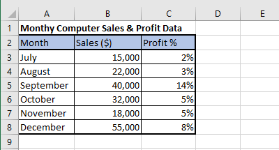
If you take a look at the Data Set as listed below, you will notice that Monthly Sales are measured in Dollars, while the Profit earned is measured in percentage (%).
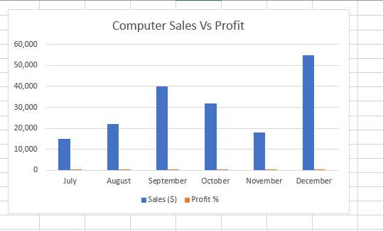
When this type of mixed data is used to create a Bar Chart in Excel, we end up with a Chart that does not represent the complete information.
In above Chart, the blue bars represent Monthly Sales ($) and the tiny Orange bars represent Profit Margins (%). While this Chart does provide fair representation of Monthly Sales figures, it hardly provides any useful information about Monthly Profits earned. This deficiency in an Excel Chart can be easily fixed by adding a Secondary Axis to accurately represent the under-represented data (Profit margin in this case). So, let us go ahead and take a look at two different methods to add Secondary Axis in a Bar Chart.
1. Add Secondary Axis Using Recommended Charts Option in Excel
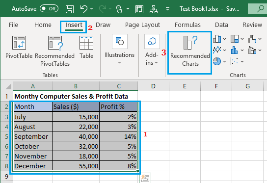
The simplest way to Add Secondary Axis to Chart in Excel is to make use of the Recommended Charts feature as available in Excel 2013 and later versions.
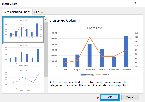
Select the Data Set > click on the Insert tab > Recommended Charts option in the ‘Charts’ section.
In the Insert Chart dialog box, go through recommended Charts in the left pane and select the Chart with a Secondary Axis.
Click on OK to close the dialogue box and you will end up with an Excel Chart having a primary and secondary axis.
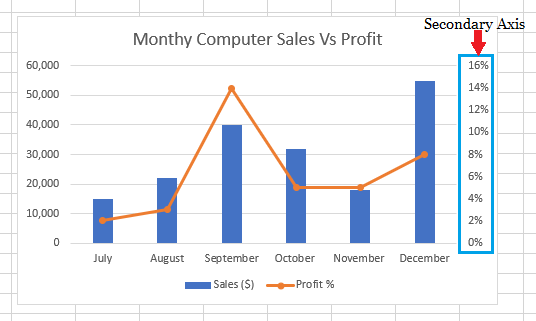
As you can see in above image, adding a Secondary Axis has led to a better representation of both Monthly Sales and Profit Margins.
2. Manually Add Secondary Axis to Chart in Excel
If you do not find a Chart with secondary axis, you can manually add a secondary axis by following the steps below.
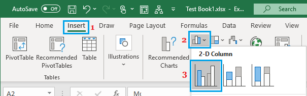
Select the Data Set > click on the Insert tab and select 2-D Clustered Column Chart option.
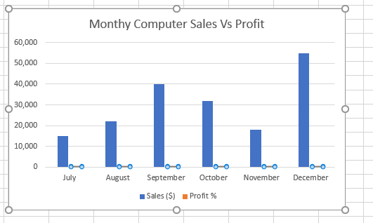
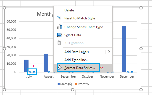
In the inserted Chart, select the Minor bars (Profit bars). If the minor bars are tiny, select the Major or Larger bars (Sales Bars) and hit the Tab key.
After selecting the Minor Bars, right-click and select Format Data Series option.
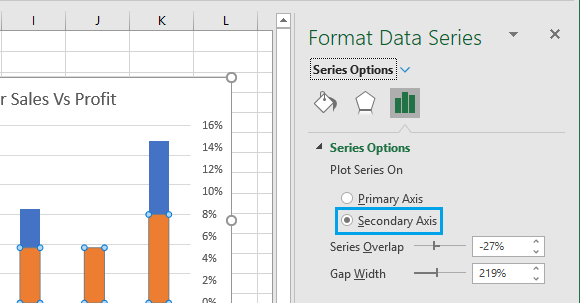
In the right-pane that appears, select the Secondary Axis option.
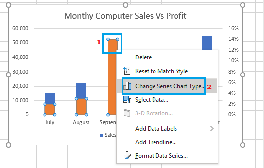
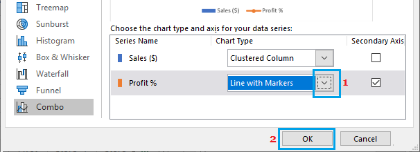
This will add a secondary axis to the existing bar chart and you will end up with two overlapping bars. 5. Now, right-click on the Profit margin bar and select Change Series Chart Type option. 6. In Change Chart Type dialog box, change the Profit Margin Chart type to Line with Markers. 7. Click on OK to save the changes. You will now have a Bar Chart with a Primary Axis representing Sales Data ($) and a Secondary Axis representing Profit Margins (%).
How to Remove Secondary Axis from an Excel Chart?
All that is required to remove secondary axis in an Excel Bar Chart is to select the secondary axis and press the Delete key.
- Select the Secondary Axis by clicking on it.
- Press the Delete Key on the keyboard of your computer Alternately, you can also right-click on the secondary axis and click on the Delete option in the contextual menu.
How to Create Gantt Chart in Excel How to Create Waterfall Chart in Excel