Create Two Pivot Tables in Single Worksheet
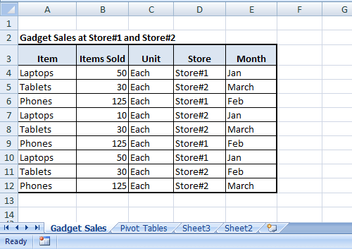
As mentioned above, the common reason for creating Two Pivot Tables in Single Worksheets is to analyze and report data in two different ways. For example, consider the following Sales Data as recorded at 2 different store locations (Store#1 and Store#2).
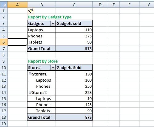
For above Sales Data, you can Create Two Pivot Table in same Worksheet, reporting or analyzing Sales Data in two different ways. For example, the First Pivot Table can be configured to report ‘Sales Data by Gadget Type’ and the second Pivot Table to report ‘Sales Data by Store’.
1. Create First Pivot Table
Follow the steps below to create the First Pivot Table to show Sales Data by Products.
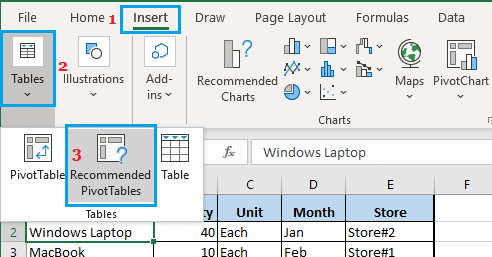
Select any Cell in the Source Data > click on Insert > Tables and select Recommended PivotTables option.
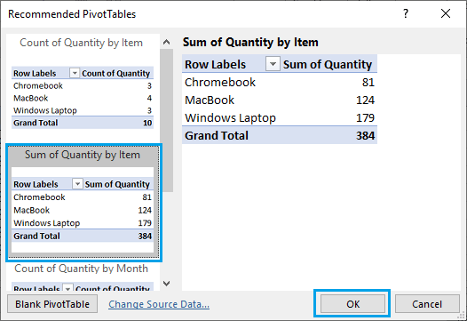
On Recommended PivotTables screen, choose the PivotTable Layout that you want to use and click on OK.
Once you click on OK, Excel will insert the first Pivot Table in a new worksheet.
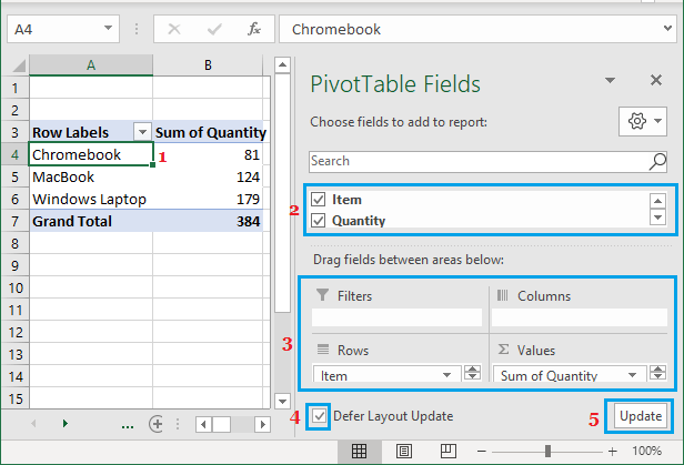
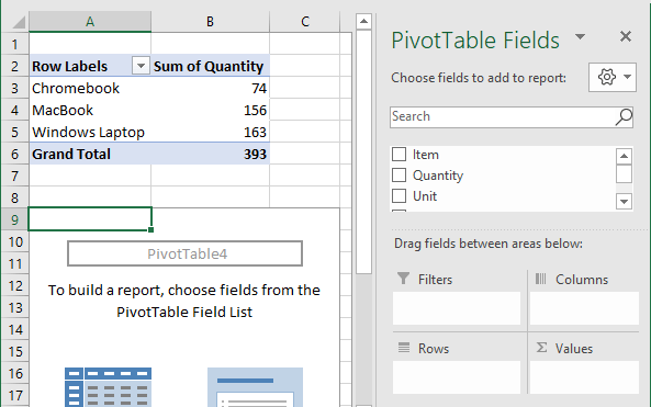
Once Pivot Table is inserted, click on any Cell within the Pivot Table and this will bring up the ‘PivotTable Fields’ List.
Modify the first Pivot Table as required by adding and dragging the Field Items between Columns, Rows and Values areas.
2. Create Second Pivot Table in Same Worksheet
Now, you can create a second Pivot Table in the same Worksheet by following the steps below.
Click on any empty cell in the same Worksheet – Make sure the Cell is away from the first pivot table that you just created.
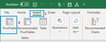
Next, click on the Insert tab and click on PivotTable option.
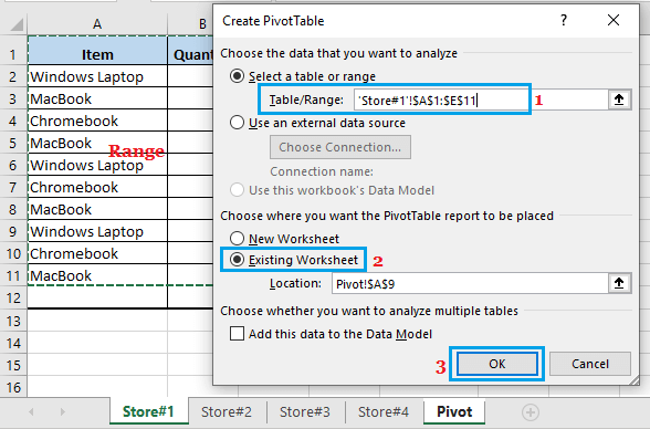
On the next screen, select Pivot Table Range, select Existing Worksheet option and click on the OK button to insert a blank Pivot Table in the same Worksheet.
Once blank Pivot Table is inserted, build the second Pivot Table as required by selecting items and dragging them between Columns, Rows and Values areas in PivotTable Fields list.
This way, you will end up with two Pivot tables on the same worksheet, reporting sales data in two different ways.
Whenever new sales are added, you can just refresh the two Pivot Tables and this will update the data in both Pivot Tables. Similarly, you can add as many pivot tables in the same worksheet as you want and report data in different ways.
How to Fix Pivot Table Report Overlap Warning
When you insert two or more Pivot Tables in the same Worksheet, you may come across Pivot Table Report overlap warning, whenever you try to make changes in the Pivot Tables.
If this happens, click on OK to close the warning message and simply space out the two Pivot Tables. You can space out Pivot Tables by inserting few blank rows (if Pivot Tables are one above another) and by inserting some blank columns (if Pivot Tables are side by side). If you are going to change Pivot Tables frequently (adding and removing fields), it is better to keep the Pivot Tables on separate worksheets.
Related
How to Create Pivot Table From Multiple Worksheets How to Add or Remove Subtotals in Pivot Table Replace Blank Cells with Zeros in Excel Pivot Table