Transpose Columns to Rows in Excel
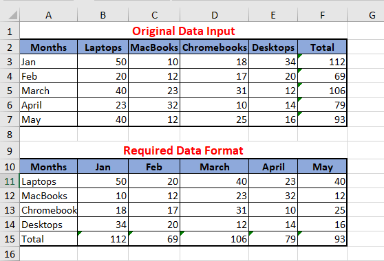
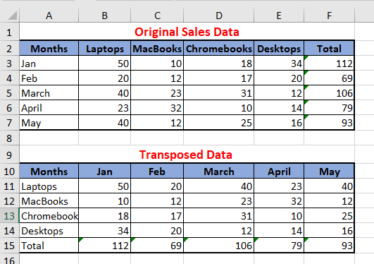
As you can see in the image below, the original data input has “Item Names” appearing as Column Labels and “Months” appearing in Rows (3 to 7). However, the actual requirement was to have the “Months” appearing as Column Labels and Items Names appearing in Rows.
When faced with such problem, many users try to re-arrange the data into required format by painfully copying and pasting data rows and columns. However, copying and pasting a large amount of data is tedious and can also give rise to errors. A better solution to fix the data is to make use of the Transpose option as available in Paste Special menu in Excel.
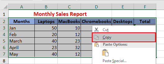
- Open the workbook containing incorrectly arranged data.
- Select the entire data set, right-click on your selection and click on Copy option in the drop-down menu.
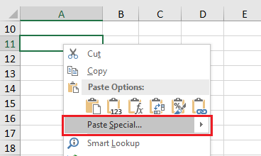
3. Next, click on a New Location in the worksheet where you want to paste the data, right-click and choose Paste Special… option in the drop-down menu that appears.
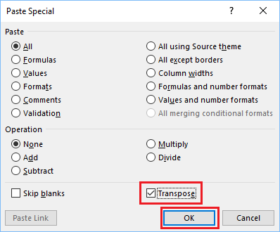
Note: Alternatively, you can use the keyboard shortcut Ctrl + Alt + V. 4. On Paste Special screen, select the Transpose option and click on the OK button.
You will now see the Transposed Data pasted in your selected location.
Note: You will be required to apply formatting as required, adjust column widths and edit column headings to suit your requirements. In above example, we have demonstrated the use of Transpose Function to rearrange data running into multiple columns and Rows. You may be pleased to know that Paste Special and Transpose option can also be used to convert a single Row of Labels into a Column, or vice versa.
How to Remove Duplicate Entries in Excel How to Start New Line in Excel Cell